Instrument Systematics Example
This notebook walks through the built-in instrument-systematics support that was originally shipped as the standalone taurex-instrumentsystematics plugin and is now part of TauREx 3. It covers:
convolution-aware binning with
FluxBinnerConv;the
OffsetSpectraloader (per-spectrum offsets, slopes and error scaling);the
OffsetSpectraContloader (offsets plus instrument response-function binning);the equivalent input-file workflow through the
spectra_w_offsetsandspectra_instrobservation keywords;a retrieval that fits those systematics together with the atmospheric parameters.
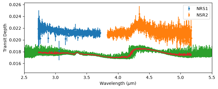
The example relies on the JWST transit data of WASP-39b NIRSpec-G395H, published in Carter et al. 2024, Nat. Ast. 8, pages 1008–1019. The data is available at: https://doi.org/10.5281/zenodo.10161743
Additionally, the Instrument Line Shape functions are required. These are available at STScI: https://jwst-crds.stsci.edu/
[22]:
import importlib
import numpy as np
import matplotlib.pyplot as plt
import _shared

_shared = importlib.reload(_shared)
build_transmission_model = _shared.build_transmission_model
## Enable if you need the opacity data.
#_shared.ensure_opacity_data(download=True)

# Use a coarse setup so the documentation notebook runs quickly.
context = build_transmission_model(
    include_cia=False,
    include_rayleigh=False,
    download=False,
    nlayers=40,
 )
tm = context['tm']
[23]:
tm.build()
[24]:
out = tm.model()
How the pieces fit together
Fitting several spectra with instrument systematics involves two sides:
Data side (the observation object). The data are corrected before they are compared with the model:
Where:
Offset_i(\(o_i\)) is the instrument’s offset.Slope_i(\(s_i\)) is the instrument’s slope.EScale_i(\(e_i\)) is the instrument’s error inflation factor.WLShift_i(\(\bar\lambda_i\)) is the instrument’s wavelength shift.
Binner side (the class, ``FluxBinnerConv``). For each spectrum i:
the native model is binned onto a fine grid at R =
wlres, padded beyond the first/last bins (this is to save compute time if the run is done at much higher resolution than the data);that fine-grid model is convolved with a Gaussian line-spread function (LSF) of width σ(λ);
it is binned onto the data bins.
The binned spectra are concatenated (same order as the files), and the χ² compares corrected data with binned model point by point.
Choosing the LSF per spectrum (path_broadening, one entry per spectrum):
entry |
when to use |
fitted parameters |
|---|---|---|
a FITS/text file ( |
calibration of LSF exist |
departure: σ = σ_file · exp(Σ c_k T_k(x)) |
|
LSF not calibrated |
ln R(λ) = Σ c_k T_k(x) |
|
do not account for LSF |
none |
\(T_k\) are Chebyshev polynomials, and x ∈ [−1, 1] spans that spectrum’s convolution grid.
broadening_ordergives the order per spectrum: 0 = a constant factor, 1 = a linear trend in ln σ, …; −1 = not fitted.With a file and no
broadening_order, the calibrated LSF is used as is.
Other functional forms. broadening_basis selects one form for all spectra of the observation: chebyshev (default), sigma_poly or resolution_poly. The default is recommended.
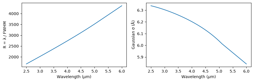
Convention: R = λ / FWHM (as defined in the STScI files), so σ = λ / (2.355 R). Use fwhm_to_sigma if you want to use another convention.
Convolution-aware binning with FluxBinnerConv
FluxBinnerConv bins a model onto one or more wavelength grids and, optionally, convolves each grid with a wavelength-dependent instrument profile. It is the building block used by the observation loaders below and supports a per-grid wavelength shift (wlshift) to absorb wavelength calibration offsets.
[25]:
## EXAMPLE OF A BIN DOWN TO R = 15k WITH A WAVELENGTH SHIFT

from taurex.util.util import create_grid_res
RES = 15000
high_res_grid1 = create_grid_res(RES, 1, 3)
high_res_grid2 = create_grid_res(RES, 3, 7.8)
from taurex.binning import FluxBinnerConv
fb = FluxBinnerConv(wlgrids= [high_res_grid1[:,0], high_res_grid2[:,0]],
        wlgrid_widths= [high_res_grid1[:,1], high_res_grid2[:,1]],
        broadening_type= 'polynomial',
        wlshift = [0, 1],
        max_wlbroadening = 0.1,
        broadening_coeffs=[[3000, 10], [3000]], ## These are the polynomial parameters.
        broadening_basis = "resolution_poly",
        factor_cut = 5,
        wlres = RES,)

x = fb.bindown(out[0], out[1])

plt.figure()
plt.plot(10000/out[0], out[1])
plt.plot(x[0], x[1])
plt.xlim(1, 7.8)
plt.show()
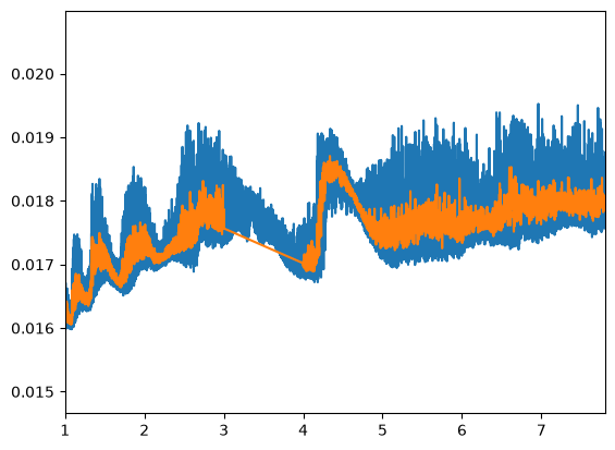
[26]:
### Now using real profiles

from taurex.util.util import create_grid_res
RES = 50000
high_res_grid1 = create_grid_res(RES, 1, 3)
high_res_grid2 = create_grid_res(RES, 3, 7.8)
from taurex.binning import FluxBinnerConv
fb = FluxBinnerConv(wlgrids= [high_res_grid1[:,0], high_res_grid2[:,0]],
        wlgrid_widths= [high_res_grid1[:,1], high_res_grid2[:,1]],
        broadening_profiles = ['../tmp/InstrumentFiles/jwst_nirspec_g395h_disp.fits',
                                                   '../tmp/InstrumentFiles/jwst_nirspec_g395h_disp.fits'],
        broadening_type = "stsci_fits",
        wlshift = [0, 0.2],
        max_wlbroadening = 0.1,
        broadening_coeffs=[[0], [-3000]], ## These are the polynomial parameters.
        broadening_basis = "resolution_poly",
        factor_cut = 5,
        wlres = RES,)

x = fb.bindown(out[0], out[1])

plt.figure()
plt.plot(10000/out[0], out[1])
plt.plot(x[0], x[1])
plt.xlim(1, 7.8)
plt.show()
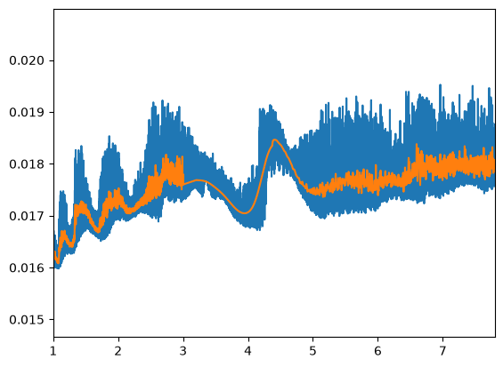
What is inside an LSF file?
STScI dispersion files give the resolving power R(λ). The binner converts it to a Gaussian σ(λ) = λ / (2.355 R). The convolution kernel is truncated at factor_cut·σ, and σ is capped at max_wlbroadening. Only use a file over the wavelength range it covers: outside that range its values are just extended flat.
[27]:
from astropy.io import fits

with fits.open('../tmp/InstrumentFiles/jwst_nirspec_g395h_disp.fits') as hdu:
    lsf = hdu[1].data
wl_lsf, R_lsf = lsf['WAVELENGTH'], lsf['R']
sigma_lsf = wl_lsf / (2.355 * R_lsf)

fig, ax = plt.subplots(1, 2, figsize=(9, 3))
ax[0].plot(wl_lsf, R_lsf); ax[0].set_xlabel('Wavelength ($\mu$m)'); ax[0].set_ylabel('R = λ / FWHM')
ax[1].plot(wl_lsf, 1e4 * sigma_lsf); ax[1].set_xlabel('Wavelength ($\mu$m)'); ax[1].set_ylabel(r'Gaussian σ (Å)')
plt.tight_layout(); plt.show()
<>:9: SyntaxWarning: "\m" is an invalid escape sequence. Such sequences will not work in the future. Did you mean "\\m"? A raw string is also an option.
<>:10: SyntaxWarning: "\m" is an invalid escape sequence. Such sequences will not work in the future. Did you mean "\\m"? A raw string is also an option.
/var/folders/4c/xrxpgpxj13s56gybbsqrpp4w0000gn/T/ipykernel_63297/2942029319.py:9: SyntaxWarning: "\m" is an invalid escape sequence. Such sequences will not work in the future. Did you mean "\\m"? A raw string is also an option.
  ax[0].plot(wl_lsf, R_lsf); ax[0].set_xlabel('Wavelength ($\mu$m)'); ax[0].set_ylabel('R = λ / FWHM')
/var/folders/4c/xrxpgpxj13s56gybbsqrpp4w0000gn/T/ipykernel_63297/2942029319.py:10: SyntaxWarning: "\m" is an invalid escape sequence. Such sequences will not work in the future. Did you mean "\\m"? A raw string is also an option.
  ax[1].plot(wl_lsf, 1e4 * sigma_lsf); ax[1].set_xlabel('Wavelength ($\mu$m)'); ax[1].set_ylabel(r'Gaussian σ (Å)')
The OffsetSpectra loader
The simplest instrument-systematics loader combines several ASCII spectra and applies a per-spectrum offset, slope and error-scale factor.
Each input spectrum automatically contributes three fittable parameters: Offset_i, Slope_i and EScale_i. This is the observation class selected by the spectra_w_offsets keyword in input files.
[181]:
from taurex.data.spectrum import OffsetSpectra

# Two WASP-39b NRS1/NRS2 spectra with per-spectrum systematics.
obs_simple = OffsetSpectra(
    path_spectra=[
        '../tmp/spectra/wasp39b_NRS1_Carter2024.txt',
        '../tmp/spectra/wasp39b_NRS2_Carter2024.txt',
    ],
    offsets=[0.0, 0.0],
    slopes=[0.0, 0.0],
    error_scale=[1.0, 1.0],
    slope_type='linear',
)

# The systematics are folded into the exposed spectrum and error bars.
obs_simple.spectrum.shape, obs_simple.errorBar.shape
[181]:
((1163,), (1163,))
[182]:
# Fittable systematics are created automatically, one set per input spectrum.
list(obs_simple.fittingParameters.keys())
[182]:
['Offset_1',
 'EScale_1',
 'Slope_1',
 'Offset_2',
 'EScale_2',
 'Slope_2',
 'WLShift_1',
 'WLShift_2']
Response-function binning with OffsetSpectraCont
When the instrument line-spread function is available (here, STScI FITS dispersion files), OffsetSpectraCont adds response-function binning on top of the offset/slope/error systematics. Its create_binner() returns a FluxBinnerConv that convolves each grid with the calibrated profile before binning. This is the observation class selected by the spectra_instr keyword.
[183]:
from taurex.data.spectrum import OffsetSpectraCont
obs = OffsetSpectraCont(path_spectra=['../tmp/spectra/wasp39b_NRS1_Carter2024.txt',
                                           '../tmp/spectra/wasp39b_NRS2_Carter2024.txt'],
                            path_broadening = ['../tmp/InstrumentFiles/jwst_nirspec_g395h_disp.fits',
                                                   '../tmp/InstrumentFiles/jwst_nirspec_g395h_disp.fits'],
                            max_wlbroadening=0.003, wlres=15000,
                            factor_cut=3, broadening_order=0,)
[184]:
obs.broadening_coeffs[0][0] = 0
inst_binner = obs.create_binner()
out_bin = inst_binner.bindown(out[0], out[1])
[185]:
obs.broadening_coeffs
[185]:
[array([0.]), array([0.])]
[186]:
plt.figure(figsize=(8,3))
plt.errorbar(obs._raw[0][:,0],obs._raw[0][:,1], yerr=obs._raw[0][:,2], fmt='.', label='NRS1')
plt.errorbar(obs._raw[1][:,0],obs._raw[1][:,1], yerr=obs._raw[1][:,2], fmt='.', label='NSR2')
plt.plot(10000/out[0], out[1])

plt.plot(out_bin[0], out_bin[1])

plt.xlim(2.5, 5.5)

plt.legend()
plt.xlabel('Wavelength ($\mu$m)')
plt.ylabel('Transit Depth')
plt.show()
<>:11: SyntaxWarning: "\m" is an invalid escape sequence. Such sequences will not work in the future. Did you mean "\\m"? A raw string is also an option.
<>:11: SyntaxWarning: "\m" is an invalid escape sequence. Such sequences will not work in the future. Did you mean "\\m"? A raw string is also an option.
/var/folders/4c/xrxpgpxj13s56gybbsqrpp4w0000gn/T/ipykernel_63297/348010052.py:11: SyntaxWarning: "\m" is an invalid escape sequence. Such sequences will not work in the future. Did you mean "\\m"? A raw string is also an option.
  plt.xlabel('Wavelength ($\mu$m)')
Per-spectrum LSF choices
Spectra prepared in different ways can be combined. Here NRS1 uses its calibrated LSF and may depart from it (order 0 = a constant scaling of σ). NRS2 is treated as if its LSF were unknown, and fits ln R(λ) as a straight line (order 1).
[192]:
obs = OffsetSpectraCont(
    path_spectra=['../tmp/spectra/wasp39b_NRS1_Carter2024.txt', '../tmp/spectra/wasp39b_NRS2_Carter2024.txt'],
    path_broadening=['../tmp/InstrumentFiles/jwst_nirspec_g395h_disp.fits', 'function'],
    broadening_order=[0, 1],
    max_wlbroadening=0.01, wlres=15000, factor_cut=5,
)

obs['Broadening_2_0'] = np.log(2700.0)

for name, p in obs.fittingParameters.items():
    if name.startswith(('Broadening', 'WLShift')):
        print(f'{name:16s} value={obs[name]: .4g}  default bounds={p[6]}')
WLShift_1        value= 0  default bounds=(-0.004059004, 0.004059004)
WLShift_2        value= 0  default bounds=(-0.003984594, 0.003984594)
Broadening_1_0   value= 0  default bounds=(-0.35, 0.35)
Broadening_2_0   value= 7.901  default bounds=(np.float64(3.912023005428146), np.float64(11.512925464970229))
Broadening_2_1   value= 0  default bounds=(-2.0, 2.0)
Input-file workflow: spectra_w_offsets and spectra_instr
The same loaders are reachable from a TauREx input file through the observation key. spectra_w_offsets selects OffsetSpectra; response functions are then attached through the [Binning] block so they can be shared with any instrument that consumes the binner. The legacy spectra_instr keyword selects OffsetSpectraCont, which wires the same broadening settings directly into the observation.
[193]:
from pathlib import Path

par_path = Path('../tmp/instruments_systematics.par')
par_path.write_text("""
[Observation]
observation = spectra_w_offsets
path_spectra = ../tmp/spectra/wasp39b_NRS1_Carter2024.txt, ../tmp/spectra/wasp39b_NRS2_Carter2024.txt
offsets = 0.0, 0.0
slopes = 0.0, 0.0
error_scale = 1.0, 1.0

[Binning]
bin_type = observed
broadening_type = stsci_fits
broadening_profiles = ../tmp/InstrumentFiles/jwst_nirspec_g395h_disp.fits, ../tmp/InstrumentFiles/jwst_nirspec_g395h_disp.fits
wlshift = 0.0, 0.0

[Fitting]
Offset_1:fit = True
Offset_2:fit = True
EScale_1:fit = True
EScale_2:fit = True
""")

from taurex.parameter import ParameterParser

pp = ParameterParser()
pp.read(str(par_path.resolve()))
obs_par = pp.generate_observation()
binner, wngrid = pp.generate_binning(observation=obs_par)

obs_par.__class__.__name__, binner.__class__.__name__
[193]:
('OffsetSpectra', 'FluxBinnerConv')
[194]:
# The observation exposes the systematics as fittable parameters, while the
# binner carries the response-function and wavelength-shift configuration.
list(obs_par.fittingParameters.keys())
[194]:
['Offset_1',
 'EScale_1',
 'Slope_1',
 'Offset_2',
 'EScale_2',
 'Slope_2',
 'WLShift_1',
 'WLShift_2']
Full-feature input file (spectra_instr)
spectra_instr is the class that supports LSF fitting, per-spectrum LSF modes and fitted wavelength shifts. Every per-spectrum keyword takes one entry per file, in the same order as path_spectra.
[38]:
# This ccan be done directly in notebook

obs = OffsetSpectraCont(
        path_spectra=['../tmp/spectra/wasp39b_NRS1_Carter2024.txt', '../tmp/spectra/wasp39b_NRS2_Carter2024.txt'],
        path_broadening = ['../tmp/InstrumentFiles/jwst_nirspec_g395h_disp.fits', '../tmp/InstrumentFiles/jwst_nirspec_g395h_disp.fits'],
        wlres=15000,
        offsets = [0,0],
        slopes = [0,0],
        error_scale = None,
        slope_type = "linear",
        broadening_type = "stsci_fits",
        wlshift = [0.0, 0.0],
        max_wlbroadening=0.003,
        factor_cut = 5,
        broadening_order = [0,0],
        broadening_basis="chebyshev",
        fwhm_to_sigma = 2.355,

)
[196]:
# Or a similar one in parfile mode

par_full = Path('../tmp/instruments_full.par')
par_full.write_text('''
[Observation]
observation = spectra_instr
path_spectra = ../tmp/spectra/wasp39b_NRS1_Carter2024.txt, ../tmp/spectra/wasp39b_NRS2_Carter2024.txt
path_broadening = ../tmp/InstrumentFiles/jwst_nirspec_g395h_disp.fits, '../tmp/InstrumentFiles/jwst_nirspec_g395h_disp.fits'
broadening_order = 0, 0
max_wlbroadening = 0.01

[Fitting]
Offset_2:fit = True
Offset_2:bounds = -1e-3, 1e-3
WLShift_2:fit = True
Broadening_1_0:fit = True
Broadening_2_0:fit = True
Broadening_2_0:bounds = 6.5, 8.5
Broadening_2_1:fit = True
''')

pp_full = ParameterParser()
pp_full.read(str(par_full.resolve()))
obs_full = pp_full.generate_observation()
type(obs_full).__name__, [k for k in obs_full.fittingParameters if k.startswith(('Broadening', 'WLShift'))]
[196]:
('OffsetSpectraCont',
 ['WLShift_1', 'WLShift_2', 'Broadening_1_0', 'Broadening_2_0'])
Retrieval with instrument systematics
The systematics parameters can be fitted alongside the atmospheric parameters. The Broadening_N_0 parameters correct the calibrated line-spread function, Offset_N absorbs baseline shifts, and EScale_N rescales the per-instrument error bars.
[39]:
from taurex.optimizer.nestle import NestleOptimizer

opt = NestleOptimizer(num_live_points=50, tol=30.0)
opt.set_model(tm)
opt.set_observed(obs)

opt.enable_fit('Offset_1')
opt.set_boundary('Offset_1', [-1e-2, 1e-2])

opt.enable_fit('EScale_1')
opt.set_boundary('EScale_1', [0.8, 5])

opt.enable_fit('EScale_2')
opt.set_boundary('EScale_2', [0.8, 5])

opt.enable_fit('Broadening_1_0')
opt.set_boundary('Broadening_1_0', [-0.35, 0.35])

opt.enable_fit('Broadening_2_0')
opt.set_boundary('Broadening_2_0', [-0.35, 0.35])

opt.enable_fit('WLShift_1')
opt.set_boundary('WLShift_1', [-0.5, 0.5])

opt.enable_fit('T')
opt.set_boundary('T', [300, 3000])

opt.enable_fit('H2O')
opt.set_boundary('H2O', [1e-12, 0.1])

opt.enable_fit('CO2')
opt.set_boundary('CO2', [1e-12, 0.1])

opt.enable_fit('planet_radius')
opt.set_boundary('planet_radius', [0.5, 2])
[40]:
res = opt.fit()
it=  1140 logz=7311.9273642154niter: 1141
ncall: 6857
nsamples: 1191
logz: 7338.058 +/-  0.727
h: 26.418
[42]:
for solution,optimized_map,optimized_value,values in opt.get_solution():
    opt.update_model(optimized_map)
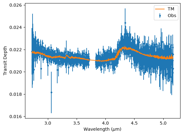
[179]:
plt.figure()
plt.errorbar(obs.wavelengthGrid,obs.spectrum,obs.errorBar, fmt='.', label='Obs')
plt.plot(obs.wavelengthGrid,inst_binner.bin_model(tm.model(obs.wavenumberGrid))[1],label='TM', zorder=10)
plt.legend()
plt.xlabel('Wavelength ($\mu$m)')
plt.ylabel('Transit Depth')
plt.show()
<>:5: SyntaxWarning: "\m" is an invalid escape sequence. Such sequences will not work in the future. Did you mean "\\m"? A raw string is also an option.
<>:5: SyntaxWarning: "\m" is an invalid escape sequence. Such sequences will not work in the future. Did you mean "\\m"? A raw string is also an option.
/var/folders/4c/xrxpgpxj13s56gybbsqrpp4w0000gn/T/ipykernel_63297/103401483.py:5: SyntaxWarning: "\m" is an invalid escape sequence. Such sequences will not work in the future. Did you mean "\\m"? A raw string is also an option.
  plt.xlabel('Wavelength ($\mu$m)')
[180]:
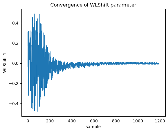
plt.figure()
plt.plot(res['solution0']['fit_params']['WLShift_1']['trace'])
plt.title('Convergence of WLShift parameter')
plt.xlabel('sample')
plt.ylabel('WLShift_1')
plt.show()
[205]:
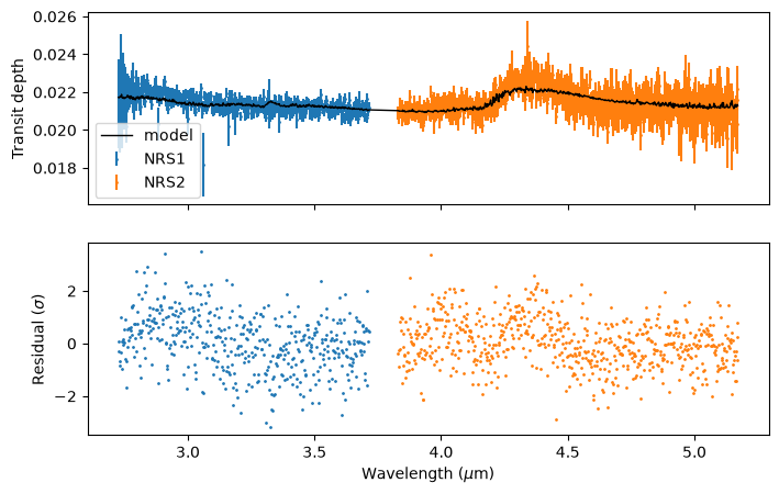
# and the fitted systematics

for name, value in zip(opt.fit_names, optimized_map):
    if name.startswith(('Offset', 'Slope', 'EScale', 'Broadening', 'WLShift')):
        print(name, value)

model_binned = opt._binner.bin_model(tm.model(obs.wavenumberGrid))[1]
edges = np.cumsum([0] + [len(r) for r in obs._raw])
fig, ax = plt.subplots(2, 1, figsize=(8, 5), sharex=True)
for i, label in enumerate(['NRS1', 'NRS2']):
    sl = slice(edges[i], edges[i + 1])
    ax[0].errorbar(obs.wavelengthGrid[sl], obs.spectrum[sl], obs.errorBar[sl], fmt='.', ms=2, label=label)
    ax[1].plot(obs.wavelengthGrid[sl], (obs.spectrum[sl] - model_binned[sl]) / obs.errorBar[sl], '.', ms=2)
ax[0].plot(obs.wavelengthGrid, model_binned, color='black', lw=1, label='model', zorder=10)
ax[0].set_ylabel('Transit depth'); ax[0].legend()
ax[1].set_ylabel('Residual ($\sigma$)'); ax[1].set_xlabel('Wavelength ($\mu$m)')
plt.show()
<>:16: SyntaxWarning: "\s" is an invalid escape sequence. Such sequences will not work in the future. Did you mean "\\s"? A raw string is also an option.
<>:16: SyntaxWarning: "\m" is an invalid escape sequence. Such sequences will not work in the future. Did you mean "\\m"? A raw string is also an option.
/var/folders/4c/xrxpgpxj13s56gybbsqrpp4w0000gn/T/ipykernel_63297/206241550.py:16: SyntaxWarning: "\s" is an invalid escape sequence. Such sequences will not work in the future. Did you mean "\\s"? A raw string is also an option.
  ax[1].set_ylabel('Residual ($\sigma$)'); ax[1].set_xlabel('Wavelength ($\mu$m)')
/var/folders/4c/xrxpgpxj13s56gybbsqrpp4w0000gn/T/ipykernel_63297/206241550.py:16: SyntaxWarning: "\m" is an invalid escape sequence. Such sequences will not work in the future. Did you mean "\\m"? A raw string is also an option.
  ax[1].set_ylabel('Residual ($\sigma$)'); ax[1].set_xlabel('Wavelength ($\mu$m)')
Offset_1 -1.6992387977442236e-05
EScale_1 1.120949778487453
EScale_2 0.9704244488598507
WLShift_1 0.0009633142673415307
Broadening_1_0 0.013356093137605052
Broadening_2_0 -0.07808122616865237
[ ]: